Discrete complexes for fluid dynamics
Ma thèse s'intitule complexes discret pour les fluides incompressible. Les complexes sont donc naturellement un objet central.
2ième passage
L'objectif est d'introduire les principaux résultats obtenu,
en particulier je vais essayer de ne pas rentrer dans les aspects les plus technique.
Je ne parlerais pas du premier chapitre de ma thèse sur les lois de Biot Savart.
Exterior calculus
-
Objects
$k$-vectors and $k$-forms

$T_x\Omega = \Lambda^1(\Omega)$
$e_1$, $\ e_2$, $\ \dots$

$\Lambda^2(\Omega)$
$e_1 \wedge e_2$, $\ \dots$
$\vdots$
$\vdots$
$\vdots$
-
Operators
-
Exterior product:
\begin{equation}\wedge: \Lambda^k(\Omega) \times \Lambda^l(\Omega) \rightarrow \Lambda^{k+l}(\Omega).\end{equation}
-
Exterior derivative:
\begin{equation}d: \Lambda^k(\Omega) \rightarrow \Lambda^{k+1}(\Omega).\end{equation}
-
Hodge star operator:
\begin{equation}\star: \Lambda^k(\Omega) \rightarrow \Lambda^{n-k}(\Omega).\end{equation}
-
Exterior product
Free alternating product satisfying \begin{equation} \alpha \wedge \beta = (-1)^{k l} \beta \wedge \alpha,\ \forall \alpha \in \Lambda^k(\Omega), \beta \in \Lambda^l(\Omega). \end{equation}
Can be seen as oriented hypervolumes.
Exterior derivative
- On functions ($0$-forms/vectors) $d$ is the differential.
- $d^2 = 0$.
- $d(\alpha \wedge \beta) = d\alpha \wedge \beta + (-1)^k (\alpha \wedge d\beta),\ \forall \alpha \in \Lambda^k(\Omega), \beta \in \Lambda^l(\Omega)$.
Hodge star
If $\Omega$ is of dimension $n$ then $ \text{dim } \Lambda^k(\Omega) = \begin{pmatrix}n\\k\end{pmatrix}. $
In particular $\Lambda^n(\Omega) \simeq \Lambda^0(\Omega)$. Given a volume form $\text{vol}_n \in \Lambda^n(\Omega)$: \begin{equation} \alpha \wedge (\star \beta) = \langle \alpha, \beta \rangle \text{vol}_n,\ \forall \alpha, \beta \in \Lambda^k(\Omega). \end{equation}
Proxy over a $3$-dimensional domain

Example (exterior derivative of a $1$-form):

Dire que c'est un complexe
Navier-Stokes equations
\begin{equation*} \begin{aligned} \frac{\partial \bvec{u}}{\partial t} - \nu \Delta \bvec{u} + \nabla p + (\bvec{u} \cdot \nabla)\bvec{u} =&\, f,\\ \nabla \cdot \bvec{u} =&\, 0. \end{aligned} \end{equation*}
- $(\bvec{u} \cdot \nabla) \, \bvec{u} = \frac{1}{2} \nabla (\bvec{u} \cdot \bvec{u}) - \bvec{u} \times (\CURL \bvec{u})$.
- $\Delta \bvec{u} = \GRAD \DIV \bvec{u} - \CURL (\CURL \bvec{u}) = - \CURL (\CURL \bvec{u})$.
\begin{equation*} \begin{aligned} \frac{\partial \bvec{u}}{\partial t} + \nu \CURL (\CURL \bvec{u}) + \GRAD P + (\CURL \bvec{u}) \times \bvec{u} =&\, f,\\ \DIV \bvec{u} =&\, 0, \end{aligned} \end{equation*} where $P := \frac{1}{2} \bvec{u} \cdot \bvec{u} + p$ is the Bernoulli pressure.
Through proxies:
We define: \begin{equation} \delta := (-1)^{n(k-1)+1} \star \DIFF \star . \end{equation}
- If $\bvec{u} \in \Lambda^1(\Omega)$ and $p \in \Lambda^0(\Omega)$, \begin{equation*} \begin{aligned} \frac{\partial \bvec{u}}{\partial t} + \nu \delta \DIFF \bvec{u} + \DIFF P + \star \big( ( \star \DIFF \bvec{u} ) \wedge \bvec{u} \big) =&\, f,\\ \delta \bvec{u} =&\, 0. \end{aligned} \end{equation*}
- If $\bvec{u} \in \Lambda^2(\Omega)$ and $p \in \Lambda^3(\Omega)$, \begin{equation*} \begin{aligned} \frac{\partial \bvec{u}}{\partial t} + \nu \DIFF \delta \bvec{u} + \delta P + \delta \bvec{u} \wedge \star \bvec{u} =&\, f,\\ \DIFF \bvec{u} =&\, 0. \end{aligned} \end{equation*}
Two complexes
De Rham:

Stokes:

Subcomplexes
$V^0$
$V^1$
$V^2$
$V^3$
$V^0_h$
$V^1_h$
$V^2_h$
$V^3_h$
$d^0$
$d^1$
$d^2$
$d^0_h$
$d^1_h$
$d^2_h$
$\pi_h^0$
$\pi_h^1$
$\pi_h^2$
$\pi_h^3$
Bounded projections
There exist some projectors $\pi_h^i : V^i \rightarrow V_h^i$ that:
- Are bounded for the graph norm: $\exists c > 0,$ $\forall v \in V^i,$ $\Vert \pi_h^i v\Vert_{V} \leq c \Vert v \Vert_{V}$ (or better for the $L^2$-norm).
- Commute with the differential operators.
Approximation properties
Errors are typically proportional to \begin{equation} E(v) := \inf_{v_h \in V_h} \Vert v - v_h \Vert .\end{equation}
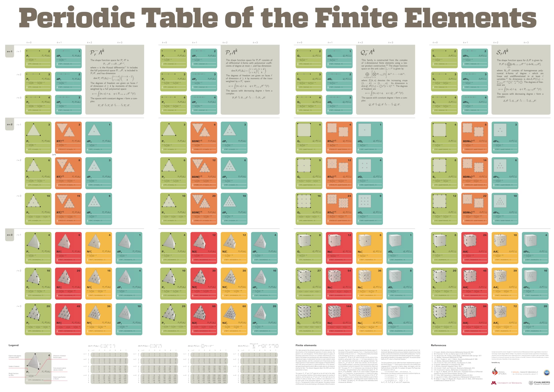
Finite Element Exterior Calculus
General principles:
Objects: Discretes spaces forming a subcomplex $V^0_h$, $V^1_h$, $V^2_h$ and $V^3_h$.
Operators: $d_h := d_{\vert V_h}$ and $\ccancel[blue]{\delta_h} := d_h^\star$.
Operators: $d_h := d_{\vert V_h}$ and $\delta_h := d_h^\star$.
$\delta_h$ is global and hard to analyse, it is replaced by $\omega^{i-1}$ such that: \begin{equation} \langle \omega^{i-1}, \sigma^{i-1} \rangle = \langle u^i, d^{i-1}_h \sigma^{i-1} \rangle, \forall \sigma^{i-1} \in V^{i-1}_h . \end{equation}
Concrete spaces:
The method is independent of the exact choice of spaces.
For the De Rham complex two families of arbitrary degree on simplicial and cubical meshes already exist.
Tools
- Hodge decomposition:

- Isomorphism of the cohomology:

Scheme for incompressible Navier-Stokes equations
Find $(\bvec{\omega},\bvec{u}, p, \phi) \in V^1_h \times V^2_h \times V^3_h \times \mathfrak{H}^3_h$ such that $\forall (\bvec{\tau},\bvec{v}, q, \chi) \in V^1_h \times V^2_h \times V^3_h \times \mathfrak{H}^3_h$,

- Well-posedness.
- Convergence of the linearized problem.
-
Preservation of structure:
- Divergence free: $\Vert \nabla \cdot \bvec{u} \Vert = 0$.
- Pressure robustness: $\bvec{\omega}$ and $\bvec{u}$ do not change when changing the source by a gradient $\bvec{f} \rightarrow \bvec{f} + \nabla g$.
- Energy: using a Crank-Nicolson discretization $\frac{\partial \bvec{u}^{n + \frac{1}{2}}}{\partial t} \approx \frac{\bvec{u}^{n+1} - \bvec{u}^n}{\Delta t}$ it holds: $\Vert \bvec{u}^{n+1} \Vert^2 = \Vert \bvec{u}^n \Vert^2 - 2 \nu \Delta t \Vert \bvec{\omega}^{n + \frac{1}{2}} \Vert^2$.
Sketch of proofs
-
Well-posedness of the underlying Stokes problem:

-
Generalization with lower order terms introducing two functions $l_3 : V^1 \rightarrow V^2$ and $l_5 : V^2 \rightarrow V^2$:
- Continuous well-posedness with a compactness argument.
- Discrete Inf-sup stability with test functions constructed from the continuous solution operator.
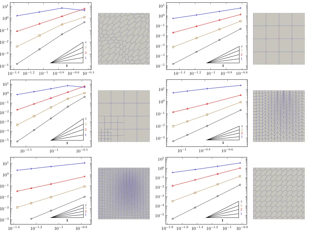
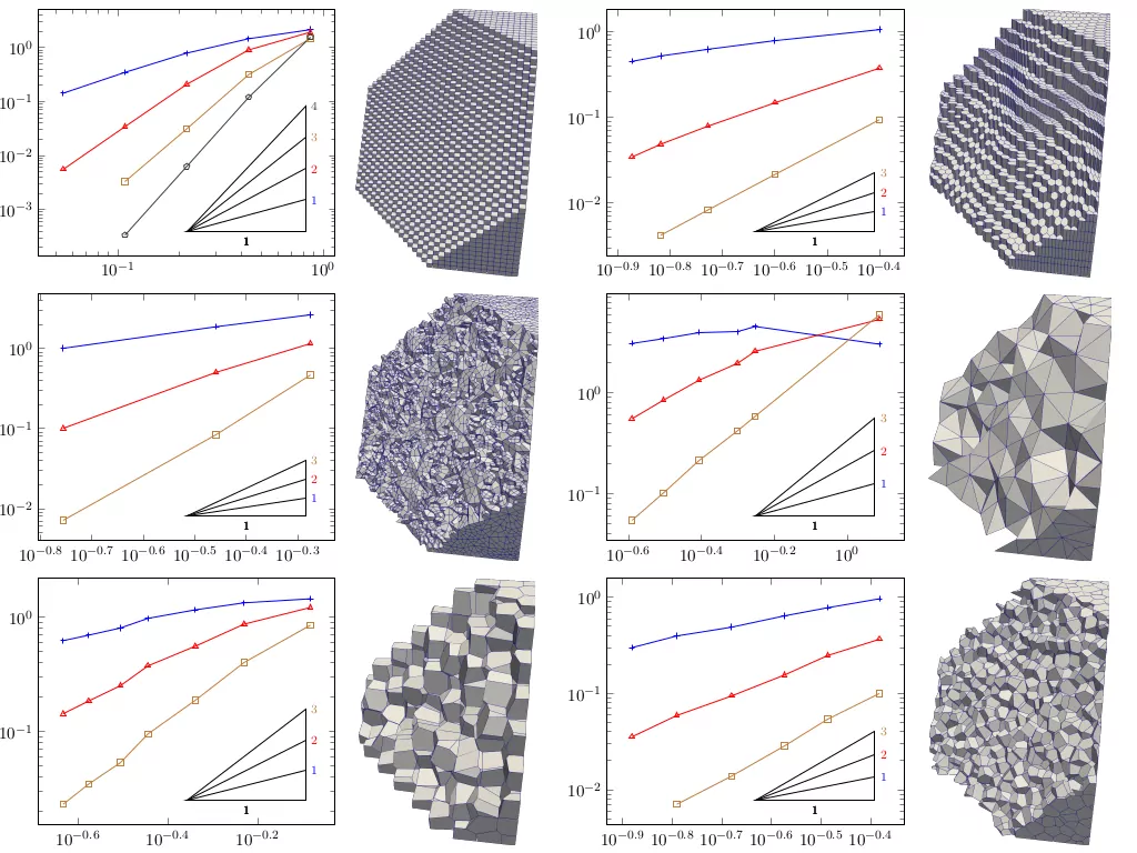
Applications
-
Convergence towards an exact solution
\begin{equation} u = \begin{pmatrix} -a (e^{a x}\sin(a y + d z) + e^{a z}\cos(a x + d y))e^{-d^2 t}\\ -a (e^{a y}\sin(a z + d x) + e^{a x}\cos(a y + d z))e^{-d^2 t}\\ -a (e^{a z}\sin(a x + d y) + e^{a y}\cos(a z + d x))e^{-d^2 t} \end{pmatrix} \end{equation}

-
Pressure-robustness
-
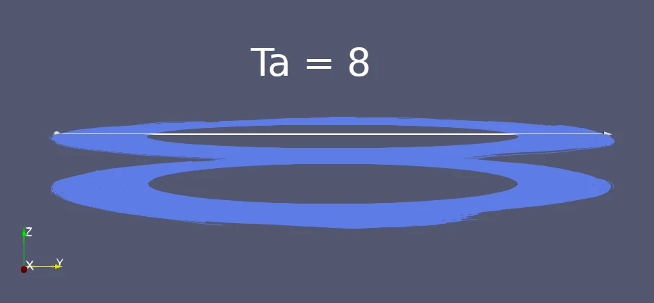
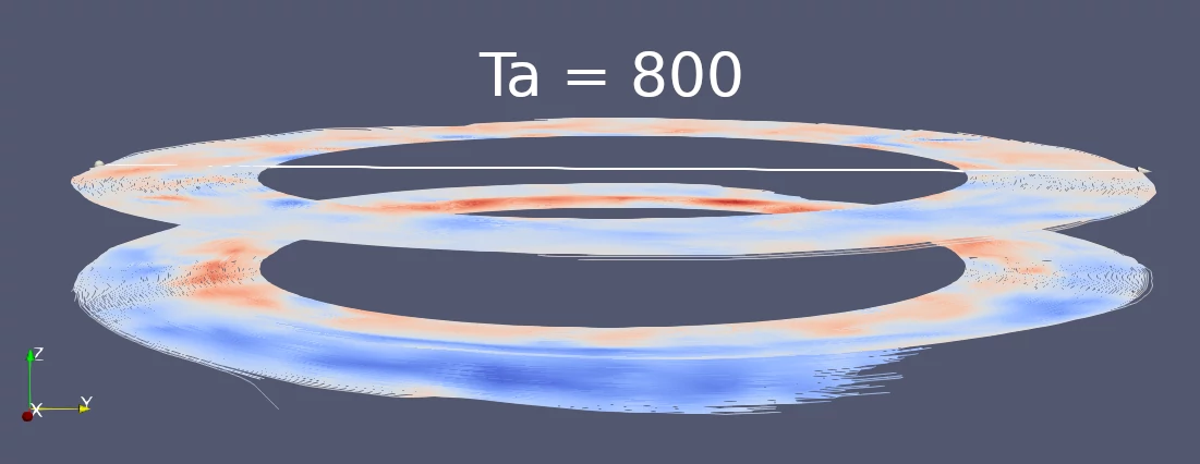
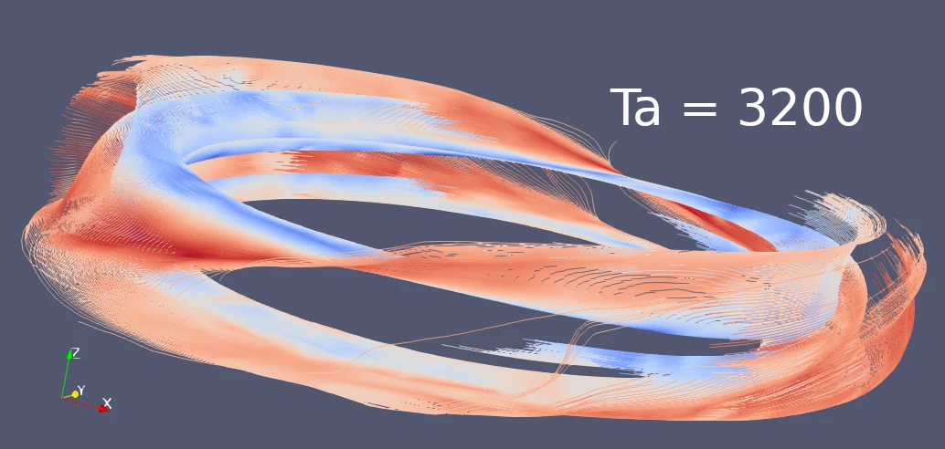
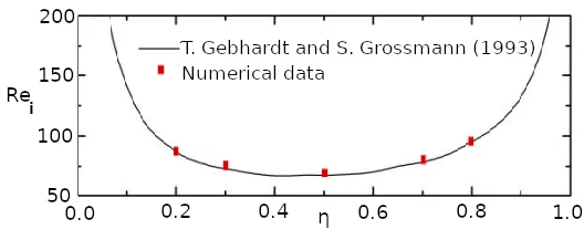
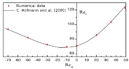
Taylor-Couette flow
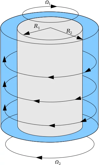
- $\eta = \frac{R_1}{R_2}$
- $Re_i = \frac{\Omega_1 R_1 (R_2 - R_1)}{\nu}$
- $Re_o = \frac{\Omega_2 R_2 (R_2 - R_1)}{\nu}$
- $Ta = \frac{(\Omega_2 - \Omega_1)^2 R_1 (R_2 - R_1)^3}{\nu}$
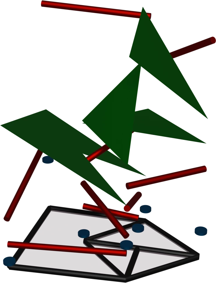
Polyhedral methods
-
Objects:
An element $\uvec{u}$ of the discrete space $\ul{X}_h$ is a collection of local functions over the cells, faces, edges and vertices: \begin{equation} \uvec{u} := \lbrace ((u_V)_{V \in \Vh}, (u_E)_{E \in \Eh}, (u_F)_{F \in \Fh}, (u_T)_{T \in \Th}) \rbrace. \end{equation} -
Operators:
-
Discrete differential: $\ul{d}_h : \ul{X}^k_h \rightarrow \ul{X}^{k+1}_h$. \begin{equation} \ul{d}_h := \lbrace ((d_V)_{V \in \Vh}, (d_E)_{E \in \Eh}, (d_F)_{F \in \Fh}, (d_T)_{T \in \Th}) \rbrace. \end{equation}

- Interpolator: $\ul{I}_h : X^k \rightarrow \ul{X}_h^k$. Typically designed to commute with the differential operator.
-
Reconstruction: $R : \ul{X}_h^k \rightarrow X^k$. Typically a right inverse of the interpolator.

-
Example on the De Rham complex
- $\int_\Omega \bvec{\omega} \GRAD q$ requires the moments on $\GRAD \Poly{k}(T)$ (completed to $\NE{k}(T)$).
- $\int_{\partial \Omega} \bvec{\omega} \cdot \bvec{n} \, q$ requires the moments on $\Poly{k}(F)$.
The local spaces for the discrete $L^2(\Omega)$ are: \begin{align} V \rightarrow&\, \emptyset \\ E \rightarrow&\, \emptyset \\ F \rightarrow&\, \emptyset \\ T \rightarrow&\, \Poly{k}(T) , \end{align}
and for the discrete $\bvec{H}(\text{div},\Omega)$: \begin{align} V \rightarrow&\, \emptyset \\ E \rightarrow&\, \emptyset \\ F \rightarrow&\, \Poly{k}(F) \\ T \rightarrow&\, \Goly{k-1}(T) \oplus \Goly{c,k}(T) . \end{align}
The discrete differential operator $D_T$ on a cell $T$ is such that \begin{equation} \int_T D_T \uvec{w}_T \, q = - \int_T \bvec{\omega}_{\Goly{},T} \cdot \GRAD q + \sum_{F \in \FT} \wTF \int_F \omega_F \, q , \quad \forall q \in \Poly{k}(T). \end{equation}
Stokes complex
- New polynomial spaces like $\Roly{k}(T)$ on tensor-valued functions.
- The data of all components on faces.
A natural space for the adjoint of $\nabla: \NE{k+1}(T) \rightarrow \bPoly{k}(T;\Real^{3,3})$

\begin{equation} \Rolyb{c,k}(T) = \begin{pmatrix} \DIV^{-1} \\ \DIV^{-1} \\ \DIV^{-1} \end{pmatrix} \circ \GRAD \Poly{0,k}(T),\quad \Rolybc{c,k}(T) = \lbrace W \in (\Roly{c,k}(T)^\intercal)^3, \Tr W = 0 \rbrace . \end{equation}
Explicit description available:
\begin{equation} \Rolybc{c,k} = \left \lbrace \begin{matrix} yz C_1 + y \gamma - z \beta \\ xz C_2 - x \gamma + z \lambda \\ xy C_3 + x \beta - y \lambda \end{matrix},\quad \begin{matrix} \lambda \in \Poly{k-2}[Y,Z],\; \beta \in \Poly{k-2}[X,Z],\; \gamma \in \Poly{k-2}[X,Y], \\ C_i \in \Poly{k-3}[X,Y,Z],\; C_1 + C_2 + C_3 = 0. \end{matrix} \right \rbrace \end{equation}
Degrees of freedom of the fully Discrete De Rham
$\uHgradh$: \begin{align} V \rightarrow&\, \Real \\ E \rightarrow&\, \Poly{k-1}(E) \\ F \rightarrow&\, \Poly{k-1}(F) \\ T \rightarrow&\, \Poly{k-1}(T) \end{align}
$\uHcurlh$: \begin{align} V \rightarrow&\, \emptyset \\ E \rightarrow&\, \Poly{k}(E) \\ F \rightarrow&\, \RT{k}(F) \\ T \rightarrow&\, \RT{k}(T) \end{align}
$\uHvh$ : \begin{align} V \rightarrow&\, \emptyset \\ E \rightarrow&\, \emptyset \\ F \rightarrow&\, \Poly{k}(F) \\ T \rightarrow&\, \NE{k}(T) \end{align}
$\uLsh$: \begin{align} V \rightarrow&\, \emptyset \\ E \rightarrow&\, \emptyset \\ F \rightarrow&\, \emptyset \\ T \rightarrow&\, \Poly{k}(T) \end{align}
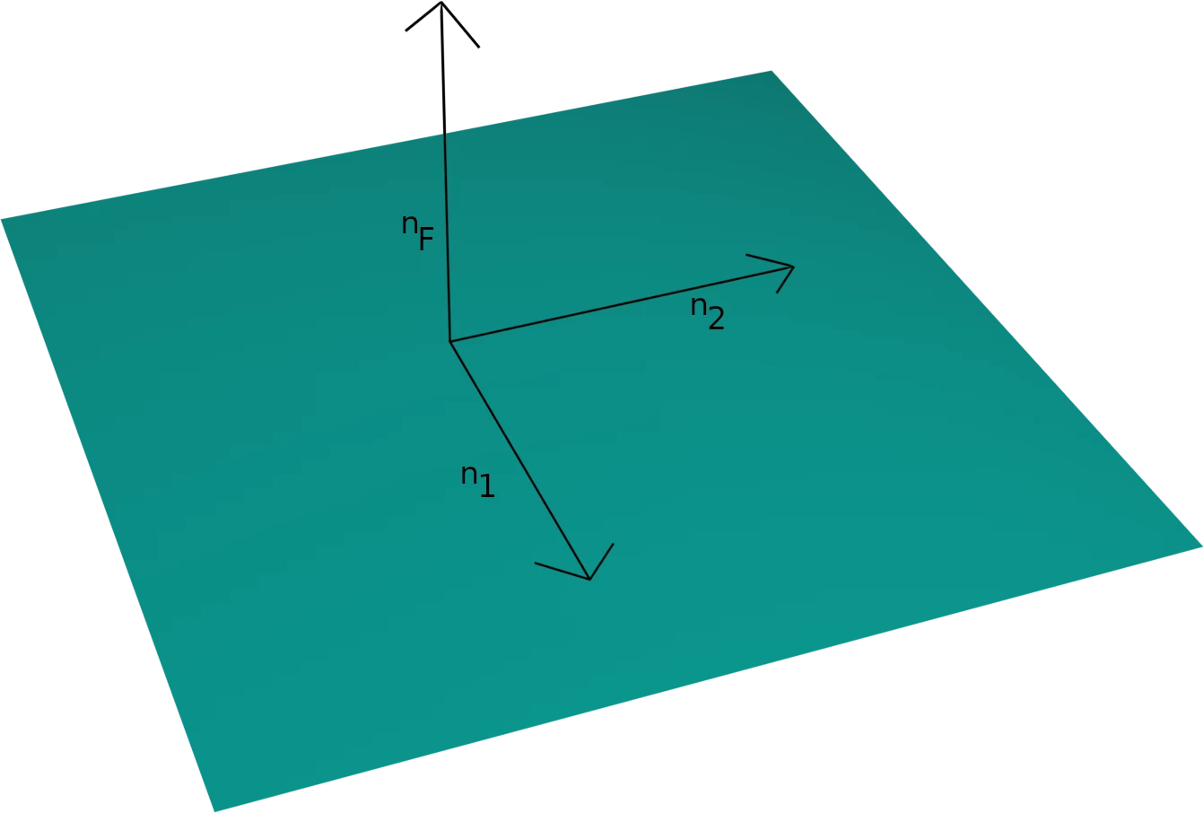
Decomposition of the curl operator
\begin{equation} \CURL \begin{pmatrix} u_1 \\ u_2 \\ u_n \end{pmatrix} = \begin{pmatrix} \partial_2 u_F - \partial_{n_F} u_2 \\ \partial_{n_F} u_1 - \partial_1 u_F \\ \partial_1 u_2 - \partial_2 u_1 \end{pmatrix} \end{equation}
\begin{equation} \underbrace{\begin{pmatrix} 0 \\ 0 \\ \partial_1 u_2 - \partial_2 u_1 \end{pmatrix}}_{\textcolor{red}{Intrinsic}} + \underbrace{\begin{pmatrix} \partial_2 u_F \\ - \partial_1 u_F \\ 0 \end{pmatrix}}_{\color{red}{Computable}} + \underbrace{\partial_{n_F} \begin{pmatrix} - u_2 \\ u_1 \\ 0 \end{pmatrix}}_{\color{red}{Extrinsic}} \end{equation}
The local spaces of $\uHcurlh$ now include: \begin{equation} V \rightarrow\, \emptyset ,\ E \rightarrow\, \begin{matrix} \Poly{k}(E)\\ \bPoly{k}(E;\Real^2) \end{matrix} ,\ F \rightarrow\, \begin{matrix} \RT{k}(F) \\ \bPoly{k}(F;\Real^2) \\ \Poly{k-1}(F) \end{matrix} ,\ T \rightarrow\, \RT{k}(T) . \end{equation}
The local spaces of $\uHgradh$ now include: \begin{equation} V \rightarrow\, \begin{matrix} \Real \\ \Real^3 \end{matrix} ,\ E \rightarrow\, \begin{matrix} \Poly{k-1}(E)\\ \bPoly{k}(E;\Real^2) \end{matrix} ,\ F \rightarrow\, \begin{matrix} \Poly{k-1}(F)\\ \Poly{k-1}(F) \end{matrix} ,\ T \rightarrow\, \Poly{k-1}(T). \end{equation}
Problem: $\uHvh$ is not smooth enough to get Poincaré inequality (equivalently the discrete $\nabla$ does not carry enough information).
We had to add a continuous $1$-skeleton on $\uHvh$ and its pre-image.
The full picture is:
$\uHgradh$: \begin{align} V \rightarrow&\, \begin{matrix} \Real \\ \Real^3 \end{matrix} \\[1em] E \rightarrow&\, \begin{matrix} \Poly{k-1}(E)\\ \bPoly{k}(E;\Real^2) \end{matrix} \\[1em] F \rightarrow&\, \begin{matrix} \Poly{k-1}(F)\\ \Poly{k-1}(F) \end{matrix} \\[1em] T \rightarrow&\, \Poly{k-1}(T) \end{align}
$\uHcurlh$: \begin{align} V \rightarrow&\, \begin{matrix} \Real^3 \\ \Real^3 \end{matrix} \\[1em] E \rightarrow&\, \begin{matrix} \bPoly{k+1}(E;\Real^3)\\ \bPoly{k}(E;\Real^3) \end{matrix} \\[1em] F \rightarrow&\, \RT{k}(F) \\[1em] T \rightarrow&\, \RT{k}(T) \end{align}
$\uHvh$ : \begin{align} V \rightarrow&\, \Real^3 \\[1em] E \rightarrow&\, \bPoly{k+1}(E;\Real^3) \\[1em] F \rightarrow&\, \begin{matrix} \RT{k}(F) \\ \bPoly{k}(F;\Real^2) \\ \Poly{k-1}(F) \end{matrix} \\[1em] T \rightarrow&\, \NE{k}(T) \end{align}
$\uLsh$: \begin{align} V \rightarrow&\, \emptyset \\[1em] E \rightarrow&\, \emptyset \\[1em] F \rightarrow&\, \emptyset \\[1em] T \rightarrow&\, \Poly{k}(T) \end{align}
Summary

Main results on $\nabla$
- Primal consistency \begin{equation} \norm{\pna ( \uIH \bvec{w}) - \bvec{w}} \lesssim h^{k+2} \seminorm[\bvec{H}^{k+2}]{\bvec{w}},\quad \forall \bvec{w}\in \bvec{H}^{k+2}(T) . \end{equation}
- Poincaré inequality For all $\uvec{w}_h \in \uHvh$ such that $\sum_{T \in \Th} \int_{T} \pna \uvec{w}_T = 0$ \begin{equation} \opnNa[h]{\uvec{w}_h} \lesssim \opnLt[h]{\uNah \uvec{w}_h}. \end{equation}
- Right-inverse for the divergence If the mesh is quasi-uniform then for all $\ul{p}_h \in \uLsh$ there is $\uvec{w}_h \in \uHvh$ such that $\Dh \uvec{w}_h = \ul{p}_h$ and \begin{equation} \opnNa[h]{\uvec{w}_h} + \opnLt[h]{\uNah \uvec{w}_h} \lesssim \normLs[h]{\ul{p}_h}. \end{equation}
-
Adjoint consistency
- \begin{equation} \AdjG(\bvec{V},\uvec{w}_h) := \sum_{T \in \Th} \left (\spLt{\uIL \bvec{V}}{\uNaT \uvec{w}_T} + \int_T \TDIV \bvec{V} \cdot \pna \uvec{w}_T \right ) \end{equation} For all $\bvec{V} \in \bvec{C}^0(\overline{\Omega}) \cap \bvec{H}^1_0(\Omega)$ such that $\bvec{V} \in \bvec{H}^{k+2}(\Th)$ and all $\uvec{w}_h \in \uHvh$, it holds: \begin{equation} \seminorm{\AdjG(\bvec{V},\uvec{w}_h)} \lesssim h^{k+1} \left ( \seminorm[\bvec{H}^{k+1}]{\bvec{V}} + \seminorm[\bvec{H}^{k+2}]{\bvec{V}} \right ) \left ( \opnNa[h]{\uvec{w}_h} + \opnLt[h]{\uNah \uvec{w}_h} \right ). \end{equation}
- \begin{equation} \AdjL(\bvec{v},\uvec{w}_h) := \sum_{T \in \Th} \left ( \int_T \TLAPLACIAN \bvec{v} \cdot \pna \uvec{w}_T + \spLt{\uNaT \uIH\bvec{v}}{\uNaT \uvec{w}_T} \right ) . \end{equation} For all $\bvec{v} \in \bvec{H}^2(\Omega) \cap \bvec{C}^1(\overline{\Omega})$ such that $\TGRAD \bvec{v} \cdot \nOmega = 0$ and $\bvec{v} \in \bvec{H}^{k+2}(\Th)$ and for all $\uvec{w}_h \in \uHvh$, it holds: \begin{equation} \seminorm{\AdjL(\bvec{v},\uvec{w}_h)} \lesssim h^{k+1} \seminorm[\bvec{H}^{(k+2,3)}]{\bvec{v}} \opnLt[h]{\uNah \uvec{w}_h}. \end{equation}
Example on the Stokes problem
Continuous solution
\begin{equation} \begin{aligned} -\mu \Delta \bvec{u} + \GRAD p =&\, \bvec{f},\\ \DIV \bvec{u} =&\, 0 . \end{aligned} \end{equation}
Weak formulation
\begin{equation} \mu \int_\Omega \GRAD \bvec{u} \tdot \GRAD \bvec{w} - \int_\Omega p\, \DIV \bvec{w} + \int_\Omega \DIV \bvec{u}\, q = \int_\Omega \bvec{f} \cdot \bvec{w} . \end{equation}Discrete formulation
\begin{equation} \mu \left ( \uNah \uvec{v}_h, \uNah \uvec{w}_h \right )_{\bvec{L}^2,h} - \sum_{T \in \Th} \int_T \DT \uvec{w} \, p_T + \sum_{T \in \Th} \int_T \DT \uvec{v}_T \, q_T = \sum_{T \in \Th} \int_T \pna \uvec{w}_T \cdot \bvec{f} \end{equation}
Energy norm
\begin{equation} \normHNa{\uvec{v}_h} := \left ( \mu \norm[\nabla,h]{\uvec{v}_h}^2 + \mu \left ( \uNah \uvec{v}_h, \uNah \uvec{v}_h \right )_{\bvec{L}^2,h} \right )^{1/2} \end{equation}
Error estimate
\begin{equation} \begin{aligned} \mathcal{E}_h (\uvec{w}_h, \ul{q}_h) :=&\, \sum_{T \in \Th} \int_T \pna \uvec{w}_T \cdot \bvec{f} + \sum_{T \in \Th} \int_T \DT \uvec{w} \, \lproj{T}{k} p \\ &\quad - \mu \left ( \uNah (\uIH[h] \bvec{u}), \uNah \uvec{w}_h \right )_{\bvec{L}^2,h} - \sum_{T \in \Th} \int_T \DT (\uIH[h] \bvec{u})\, q_T \\ =&\, \AdjG(p \ID, \uvec{w}_h) - \stLt{\uNaT \uvec{w}_T}{\uIL (p \ID)} - \mu \AdjL(\bvec{u},\uvec{w}_h)\\ \lesssim&\, \, h^{k+1} \left ( \mu^{\frac{1}{2}} \seminorm[\bvec{H}^{(k+2,3)}(\Th)]{\bvec{u}} + \mu^{-\frac{1}{2}} \seminorm[H^{k+1}(\Th)]{p} + \mu^{-\frac{1}{2}} \seminorm[H^{k+2}(\Th)]{p} \right ) \normHNa{\uvec{w}_h} \end{aligned} \end{equation}